[ live NDSI threshold — loading the real MODIS crop ]
01
Here’s a snow map
This is a crop from MODIS — the imaging spectrometer flying on NASA’s Terra and Aqua satellites. Snow is bright where visible light hits it and dark in the shortwave infrared. That gap between two bands, band 4 (visible) and band 6 (1.6 µm), is what separates snow from cloud and bare ground.
The ratio is called NDSI, the normalized difference snow index, and NASA has run a version of it operationally since 2000. Drag the threshold below off the standard cutoff of 0.4 and watch the mask move — turning a continuous quantity into a binary map is never as clean as one number implies.
NASA doesn’t actually ship a raw NDSI image — the operational product is MYD10_L2 (Terra’s is MOD10_L2), and its NDSI_Snow_Cover field is a byte per pixel: 0–100 is a snow-cover percentage, and everything above that is a status code — cloud, water, night, missing data. Below is that exact product, for this exact crop, straight from NSIDC — not a re-derivation — with the real legend it ships with.
[ real MYD10_L2 classification + legend — loading ]
[ detector toggle — loading the real MODIS crop ]
02
Here’s the broken sensor in the way
MODIS on Aqua has 20 physical detectors dedicated to band 6, one per scan line. Most failed shortly after launch — in this scene, only 8 of the 20 are still reading real data; the rest are stuck on a constant value. Toggle detectors off below and watch the striping return. This is the real damage pattern on Aqua, not a simulation.
NASA’s operational fallback swaps in band 7 (2.1 µm) instead. It’s spectrally close, but not close enough — snow/cloud contrast is measurably weaker there, and the standard Aqua snow product eats an accuracy hit as a result.
Worth separating two things that look similar: this is dead-detector failure, not the faint striping every MODIS band has from small calibration differences between otherwise- working detectors. That second kind gets removed with per-detector histogram matching before any of these images are even generated — standard MODIS preprocessing, not specific to this project — so what you’re seeing here is the real fault, not leftover noise.
[ band 6 vs. band 7 — loading the real MODIS crop ]
[ restoration wipe — loading real regression coefficients ]
03
Here’s how we fixed it
Instead of falling back to a worse band, predict the missing band 6 value directly from a small neighborhood of pixels in the bands that still work — a linear regression fit against the detectors that survived, applied to the ones that didn’t. This was work I did my part of at CCNY, and a version of it now runs in NASA’s operational Collection 6 Aqua snow product.
It’s cheap enough that this runs live, right now, in your browser — not a precomputed image. The wipe below shows the visible effect: every dead-detector gap (red) filled in. (Simplified from the published method: two predictor bands instead of five, one global fit instead of overlapping tiles, same 5x5 window. Close enough to be honest, light enough to ship.)
[ regression inspector — loading real coefficients ]
None of this is trustworthy without a way to check it — and Aqua alone can’t provide one. Its band 6 is permanently gone, so there’s no real answer on Aqua itself to compare a restoration against. What actually makes the fix credible is Terra: the other MODIS satellite, same instrument, band 6 fully intact. That makes the real test possible — hide Terra’s real band 6 behind the exact same 12-of-20 damage pattern Aqua actually has, restore it, and check the result against the real value Terra still has on file. This is the validation the original QIR paper ran, not something new for this site.
[ Terra validation: damaged / restored / real — loading ]
[ break it yourself — loading Terra’s real band 6 ]
04
Here’s why you can’t have one every day
A single satellite crosses any given point roughly once a day at best. Cloud cover blocks the optical view outright — across most regions, a large share of days at a given location are cloud-obstructed. A snow map that can’t refresh daily isn’t much use for hazard response, hydrology, or reservoir operations, all of which run on daily-to-weekly decisions.
MYD10_L2 carries its own cloud flag — value 250, wired in from NASA’s cloud mask — so below isn’t illustrative, it’s real: eight consecutive Aqua passes over this same region, each with that day’s actual cloud flag laid over that day’s actual scene. One look a day, whether or not that day’s look is any good.
Cloud cover isn’t a constant tax, it’s a coin flip that changes daily and independently of the satellite’s schedule — some of these days are nearly unusable, others (like the one behind step 1) are clean. And even a perfectly restored sensor doesn’t fix this: the gap above is about coverage, not sensor health — which is exactly the problem the idea below is aimed at.
[ a week of real passes — loading ]
[ weekly composite — loading eight real MYD10_L2 passes ]
05
Here’s the map I actually built
Looking back at those cloud masks, two things stand out. First, cloud obstruction is a structural limit of any reflectance- or radiance-based instrument, not a quirk of this one sensor — optical and near-infrared imagers simply can’t see through cloud, however well they’re calibrated. Second, cloud and snow (or cloud and ice) are close enough in visible/near-infrared reflectance that a classifier sometimes can’t tell them apart — real misclassification, not just an honestly-labeled gap.
That’s the case this was actually built to handle. Between 2015 and 2016, with colleagues at CCNY and NOAA’s National Ice Center, I built MISIC (Microwave/Imager Sea Ice Classifier): a real fusion algorithm, not a sketch. It takes a MODIS or VIIRS optical pass, pulls in the closest AMSR-2 passive-microwave overpass, and uses the microwave to confidently seed ice/water training regions through cloud that would otherwise mask the scene — then fits a per-scene classifier to resolve the rest at the optical instrument’s full resolution, not microwave’s coarser one. Multiple passes in a day get merged into one cloud-gap-free daily map.
Checked against Landsat 8 on six real scenes, it matched MODIS’s own operational ice product on accuracy while classifying 57–91% more of each scene — the pixels MODIS’s cloud mask simply gave up on. In one MODIS pass, MODIS’s own product misclassified a swirl of real mixed ice as solid cloud; this algorithm read it correctly. Run daily over the Beaufort Sea’s October 2015 freeze-up, its ice-extent time series tracked the operational products (IMS, OSI SAF, CMC) it was being compared against, while classifying through cloud that covered 25–60% of the region on a given day.
Optical pass
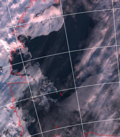
VIIRS true color at 11:37 UTC. Full optical resolution, but sea ice and cloud look almost the same.
Figure 2 · VIIRS pass at 11:37 UTC, western Ross Sea, 2016-01-16
MISIC’s real architecture, redrawn from the paper. Click any stage to see the paper’s own image of it — every image is the same place on the same day, western Ross Sea, 2016-01-16. The per-pass steps are the paper’s own figures; the daily steps are rebuilt from that day’s real satellite passes.
It’s real, working code — the National Ice Center evaluated it for operational use. What it isn’t is finished: the paper went through peer review at Remote Sensing (MDPI), and I never completed the revision, so it was never actually published. I’m hosting the manuscript myself instead — read or download it here, unrevised, exactly as it went through review. And the daily merge step has a real weakness of its own: during rapid freeze-up or melt, combining several passes sometimes loses fine ice-floe detail that a single pass gets right 4— a tradeoff I never fully resolved.
And this isn’t a mockup of what it might have looked like — these are the paper’s own real outputs, answering two questions directly: how did fusing several passes actually build one daily map, and did it actually fix the misclassification problem from earlier in this piece?
How multiple passes fuse into one daily map — Ross Sea, 2015-12-02 (the paper’s own example, a different day and area from the diagram above)
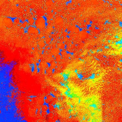
Pass 1 — 00:41 UTC
VIIRS, false-color feature space
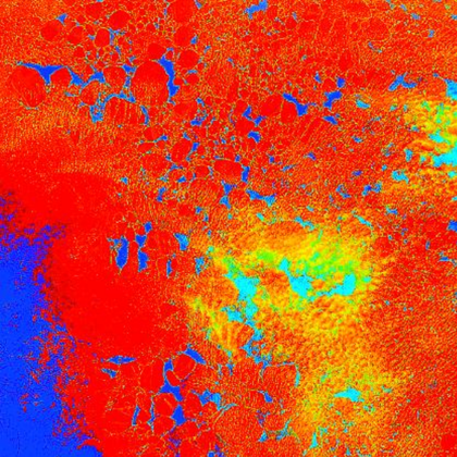
Pass 2 — 02:19 UTC
same region, cloud already moved
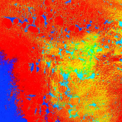
Pass 3 — 04:02 UTC
a third, differently clouded look
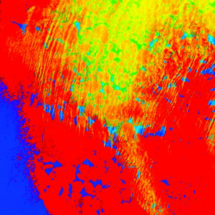
Pass 4 — 18:45 UTC
MODIS Terra, hours later
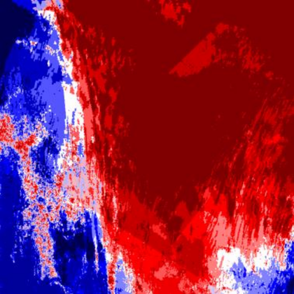
Cloud fraction, that day
dark red: obscured every pass; blue: clear
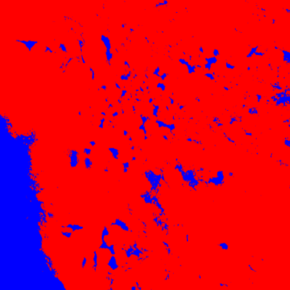
That day's fused map
every pass merged — red: ice, blue: water
Did it fix the cloud/snow misclassification? — a real case where MODIS got it wrong
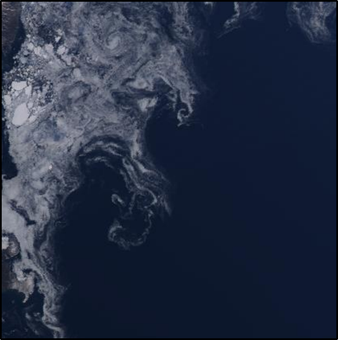
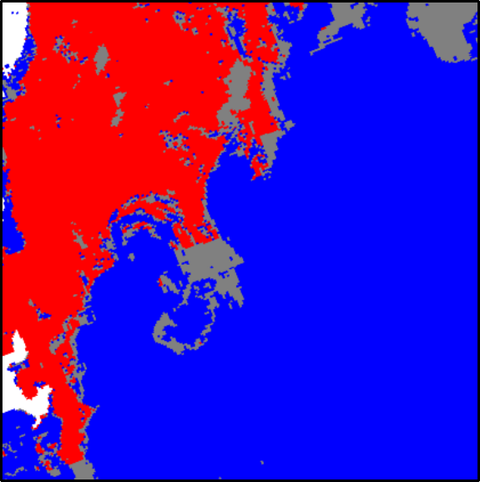
MODIS Aqua, 2015-09-15 (Figure 9). The swirl under the lens is real mixed ice — switch layers to see who calls it cloud.
Real figures from the paper (Figures 4 and 9) — not redrawn, not simulated.
Daily ice fraction, Beaufort Sea freeze-up, Oct 1–15 2015 — MISIC against IMS, NIC, OSI SAF, and CMC.
Redrawn from the paper’s real Figure 10 — values digitized from its own axes, not invented.
In retrospect, fusing heterogeneous sources with different resolutions, latencies, and reliabilities into one answer you can defend is the same problem in remote sensing and in document retrieval.